Why Should You Install a Solar Energy Meter | Usage Tracking, Billing Accuracy, System Monitoring

Installing a solar meter (bidirectional meter) is critical to protecting the return on your solar investment.

It tracks both generation and consumption in real time down to each kilowatt-hour (kWh), helping you optimize how you use electricity and typically save an additional 10% to 15% on your power bill.

At the same time, it records your surplus power exports with precision, reducing billing errors caused by utility estimates and ensuring every bill credit is counted accurately.

It also enables 24/7 system monitoring. If shading or equipment faults cause your panels' efficiency to drop abnormally, you can receive an alert right away and stop losses early.

Usage Tracking

Reading the Numbers

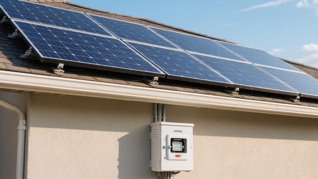
A 200-amp bidirectional meter installed inside the main distribution panel captures AC voltage and current data as often as every 1.5 seconds.

A standard set of bidirectional current transformers clamped onto a 120V/240V split-phase line can keep the maximum measurement error within a 0.5% statistical variance.

Over a full 24-hour solar cycle, the meter's built-in 16MB storage chip can retain up to 90 days of electricity usage samples recorded at 15-minute intervals.

The daily kWh figures displayed in the mobile app are calculated by the underlying system from more than 57,600 instantaneous power values per day, then averaged into a daily total.

When the inverter converts DC electricity into 60 Hz AC power, the energy tracking module records the total output precisely and subtracts the inverter's own 2 W to 5 W nighttime standby loss.

From 6:00 a.m. at sunrise to 7:00 p.m. at sunset, the system divides each hour into four independent 15-minute statistical intervals, separately measuring the kWh exported to the grid and the kWh consumed inside the home.

When a 12,000 BTU air conditioner starts up, the meter's current sensor can capture an inrush peak load of up to 15 amps within 0.1 seconds.

Identifying Usage Patterns

A full 12 months of load tracking data shows that a family of five typically reaches its highest daily electricity use in July, at around 45 kWh per day.

· Between 7:00 a.m. and 9:00 a.m., if two 1,500W hair dryers and one 800W coffee maker run at the same time, they create a sustained two-hour high-consumption window that accounts for 12% of the day's total electricity profile.

· From 12:00 p.m. to 3:00 p.m., the solar array reaches its maximum output of 4,500 W to 5,000 W. If a 200 W refrigerator is running indoors during that period, the meter will show that more than 90% of the electricity is being exported back to the grid at 240 V.

· During the evening peak from 5:00 p.m. to 9:00 p.m., when the solar UV index falls below 2, PV output drops sharply to below 500 W. A 3,000W electric oven plus a 4,000W dryer can drive grid-purchased electricity up by 300%.

By comparing fluctuations across three different time periods, the meter's cumulative kWh curve quantifies the household's daily usage pattern and calculates the absolute gap between a 25 kW daytime peak demand and a nighttime low of under 1 kW.

Over a standard 30-day billing cycle, 5-minute high-precision sampling can improve demand-side management efficiency by 18% to 22%.

If you move a dishwasher that uses 2.5 kWh per day from 8:00 p.m. to 1:00 a.m., the 1.25 kWh consumed during its 60-minute run can be covered 100% by real-time solar generation.

Calculating the Right Ratio

In the system log, the self-consumption ratio, which carries a 60% weighting parameter, identifies how much of a monthly total of 800 kWh is used directly on site and therefore incurs $0 in grid charges.

Using a communication protocol with 1% accuracy, the meter overlays 24 hourly generation data packets with hourly consumption bar charts and performs a regression analysis to calculate the correlation coefficient between the two variables.

If an 8 kW system generates 11,000 kWh per year, but no 0.1-second real-time tracking is installed, as much as 7,500 kWh, or 68%, could be exported to the grid at a low wholesale price of $0.04 per kWh.

By reviewing historical charts from the past 180 days, an operator can raise an initial 32% self-consumption rate to the 55% sweet spot.

After adding a 9.6 kWh usable LFP home cell, the meter's tracking system will automatically detect that the solar array still has 1,500 W of surplus output at 4:00 p.m. and charge that excess energy into the cell bank at up to 30 amps.

When the cell drops from 100% to its minimum discharge-protection level of 20%, the tracking record will clearly show that 7.6 kWh per day of high-priced peak electricity purchases has been replaced by self-generated clean energy at zero marginal cost.

Over the first 36 months of operation, a project with an initial budget of $18,000, supported by an underlying 0.5-second monitoring model, can shorten its payback period by 24 months, reducing a 9.5-year return timeline through annual gains that increase at a rate of $1,200 per year.

Billing Accuracy

Is the Billing Accurate

A Class 0.5 high-precision solar meter installed next to a 200-amp panel breaks the utility's 30-day billing cycle into 2,592,000 independent one-second calculation intervals.

In a standard North American home using 120V/240V split-phase AC, there are typically 15 to 20 days per month when solar generation exceeds the home's instantaneous internal load.

When a 5,000W solar array is running at full output, the meter's built-in current transformer can calculate every 1 watt exported at 240V, using a starting-current threshold as low as 10 mA.

A smart grid typically sends kWh readings to the utility backend only every 15 or 60 minutes, and a 1.5% to 2.5% packet loss rate can mean some of your exported energy is never fully recorded.

By checking the meter's internal flash memory, which can store up to 60 months of data, you can verify 450 kWh of monthly exported power down to 0.01 kWh precision.

Whenever the grid voltage shifts by 2% from the standard 240V down to 235.2V, the solar meter's built-in DSP digital signal processor can detect the reverse rate of current change within 0.05 seconds.

Mechanical utility meters and older-generation smart meters can have a non-start blind zone of up to 3% when reverse export power is below 100W.

A $180 solar meter with a low startup current of just 0.01 A can begin recording trickle exports to the grid at a rate of 0.05 kW as early as 6:30 a.m., when solar irradiance is only 50 W/m².

Checking the Fine Print

Under time-of-use pricing, 4:00 p.m. to 9:00 p.m. is billed as the peak period at $0.45 per kWh, while 9:00 p.m. to 4:00 p.m. the next day is billed at the off-peak rate of $0.12 per kWh.

A dedicated solar meter equipped with a real-time clock module can keep its cumulative monthly time drift compressed within an extremely small error band of ±0.5 seconds.

During the 60-minute sunset window from 4:00 p.m. to 5:00 p.m., solar panels can still sustain an output of 800W to 1,200W.

Selling the 1 kWh generated during that hour to the grid at $0.45 instead of $0.12 at noon yields 275% more cash value.

If the utility's meter suffers a 2-hour timing delay because of network congestion, that same 1 kWh could be incorrectly assigned to the $0.12 off-peak billing window.

Providing a CSV spreadsheet containing 86,400 timestamped power readings can help the utility correct more than 98% of billing-window misalignment issues within 3 to 5 business days.

Recovering just 5 kWh of peak-rate discrepancy per month can bring back $19.80 in pure profit over a full 12-month billing cycle.

In regions using three-tier pricing, the first 500 kWh per month is billed at $0.15 per kWh, while usage above 500 kWh and up to 1,000 kWh jumps to $0.28 per kWh.

The meter's 15-minute normal distribution charts can precisely lock in the final reading at 11:59 p.m. on day 30.

If the utility meter reader delays the reading cycle by 3 days because of a holiday, your usage could rise from 490 kWh to 540 kWh, forcing you into the higher $0.28 second-tier rate.

A digitally signed 30-day standard-cycle calendar report generated by the solar meter backend can fully overturn an improper 33-day utility billing span and cut the total bill by more than 12%.

Recovering Your Money

From March to May each year, daily sunlight increases from 10 hours to 13 hours, and a residential solar system can generate roughly 40% of its annual net-metering bill credits during that period.

A 10 kW system operating at 98% inverter efficiency in spring can deposit $150 to $200 in utility bill credits each month.

By July and August, if three 1.5-horsepower air conditioners run for 8 hours a day, monthly household electricity usage can surge to 1,200 kWh.

At an average retail electricity price of $0.25 per kWh, a monthly bill of $300 can completely consume 100% of the bill credits accumulated in spring.

When the overhead service cable heats up in 35°C summer weather, increased conductor resistance can cause a line-loss rate of 1.5% to 2.5%.

If the solar meter is installed within one meter of the inverter, the exported energy it measures is often 10 to 15 kWh per month higher than the amount recorded by the utility meter mounted on the outdoor pole.

Over a full 20-year system life, a measurement variance of 12 kWh per month can accumulate into a hidden negative asset of 2,880 kWh.

Assuming electricity prices rise at a 3% compound annual rate over 20 years, the 0.2% billing accuracy gain from a $250 hardware investment can recover more than $900 in hidden financial losses by month 240.

System Monitoring

Watching for Equipment Aging

Solar panels are typically rated for an initial degradation of 2% to 3% in the first year, followed by 0.5% per year over the next 24 years.

A monitoring meter mounted on the garage wall continuously reads the product of inverter-side DC voltage and AC current over 24 hours a day, building a lifecycle data archive that spans 300 months.

An 8 kW array made up of 20 monocrystalline 400 W modules should theoretically generate 12,000 kWh in its first 365-day full-load cycle.

By May 1 of year 6, the meter's built-in comparison algorithm can pull the historical irradiance record for the same date at 1,000 W/m² and determine that the system's actual peak power has fallen from 7,800 W initially to 7,410 W.

If the absolute degradation reaches 5%, exceeding the 4.5% allowable variance specified in the manufacturer's linear warranty, the backend system can send a 0.1 MB alert packet to your mobile app within 3 seconds.

A string inverter rated at 97.5% conversion efficiency, after running for 40,000 hours, may see its AC output efficiency fall below 95% because of thermal aging in the internal IGBT transistors. The monitoring module records that 2.5% conversion deviation as often as once every 5 minutes, and over a 30-day billing cycle, it can quantify 85 kWh of invisible loss caused by hardware aging. At $0.20 per kWh, that amounts to a monthly paper loss of $17.00.

Detecting Failed Modules

A rooftop 350V high-voltage DC line that remains exposed to extreme temperatures from -20°C to 60°C for long periods can cause the waterproof rubber seals inside MC4 connectors to develop tiny thermal expansion cracks of about 0.2 mm by month 48.

If rainwater intrusion causes insulation resistance to fall from the standard 1 MΩ to 50 kΩ, the meter's leakage-detection sensor can capture an abnormal leakage current above 30 mA within 0.05 seconds.

Before the 240V AC grid-tie switch is disconnected, the high-frequency sampled current transformer permanently writes the 0A fault cliff curve into an 8MB flash chip.

In a single string of 10 panels, if one of the three bypass diodes inside a single panel is damaged by reverse current, that panel's output voltage can instantly drop from 35V to 23V.

The total string voltage then falls from a normal 350V to 338V, and the meter's 1-second refresh voltage waveform can detect that subtle 12V difference.

Without millisecond-level monitoring, 338V may still be enough for the inverter to continue exporting power, yet the system can quietly lose 1.5 kWh per day. During a 90-day high-production summer period, that adds up to 135 kWh, or $33.75 in silent financial loss.

Monitoring Temperature Closely

The temperature sensitivity of solar cells is quantified by a negative temperature coefficient of 0.35% power loss for every 1°C increase.

When a July heat wave pushes the outdoor temperature to 38°C, solar panels mounted on a black asphalt-shingle roof can see surface temperatures soar to 65°C.

Compared with the standard test condition of 25°C, that 40°C temperature gap multiplied by the 0.35% coefficient results in a hard physical loss of 14%.

The meter's microprocessor feeds every 15-minute ambient-temperature reading into its internal multivariable regression formula and calculates that a 400W panel can produce no more than 344W at 2:00 p.m.

Combined with cooling data from a rooftop anemometer showing wind speeds of 5 m/s, the monitoring system also calculates how airflow changes within the 4-inch installation gap between the roof and the panels.

At an outdoor temperature of 38°C, if the meter shows that a single panel is producing only 300 W, far below the theoretical 344 W, the resulting 25% severe deviation indicates that more than 60% of the physical cooling channel behind the array is blocked by leaves or a bird's nest.