What time of year is best for solar panels?
Spring is the optimal season for solar power generation. Although summer has the longest daylight hours, once the panel temperature exceeds 25°C, the photoelectric conversion efficiency drops by approximately 0.4% for every 1°C increase.
Therefore, May, with its moderate temperatures, often reaches the peak of annual power generation.
In practice, it is recommended to adjust the panel tilt angle to your local latitude ±15 degrees during the change of seasons to maximize sunlight capture.
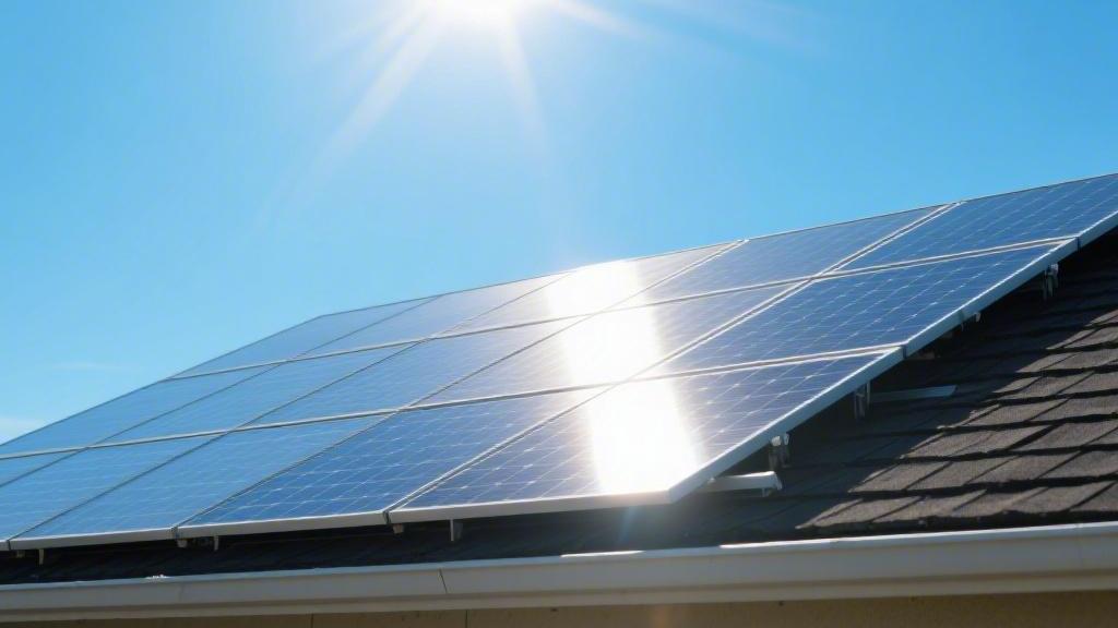
The Best Time for Efficiency
Looking at Conversion
The nominal photoelectric conversion efficiency of a single N-type TOPCon module with a rated power of 400 watts (W) under standard physical test conditions (1,000 W/m² irradiance, 25°C test temperature, AM1.5 spectral parameters) is typically 22.4%. Throughout April and May in spring, the daily average solar radiation fluctuates roughly in the range of 5.5 to 6.5 kWh/m²/day. Sampling statistics from meteorological bureaus show that the median number of rainy days in these two months is less than 7 days, and the outdoor relative humidity consistently remains in the optimal parameter range of 40% to 55%.
l When environmental humidity is below 60%, the physical light transmittance on the surface of high-voltage glass panels can be sustained at a peak of over 98.5% for a long time.
l The quantum conversion efficiency of monocrystalline silicon wafers absorbing photons to generate electron-hole pairs reaches an optimal ratio of 0.92 in spring.
l The operation response time of the system inverter's Maximum Power Point Tracking (MPPT) algorithm under stable spring lighting is generally less than 50 milliseconds, and its actual tracking accuracy breaks through the 99.9% precision ceiling.
A 10 kW residential system consisting of 25 panels has an extremely high probability of reaching a median daily power generation of 45 to 55 kilowatt-hours (kWh) in spring. Calculated at a grid bill rate of $0.25 per kWh, the system's daily financial budget return can hit a monetary yield of $11.25 to $13.75.
[Image of solar panel temperature coefficient graph] Cooling Down and Reducing Loss
The power temperature coefficient inside solar cells generally falls within a negatively correlated slope range of -0.30%/°C to -0.40%/°C. When the absolute maximum outdoor air temperature soars to 35°C in July, the surface operating temperature of dark-colored panels after absorbing thermal radiation usually climbs to a high extreme of 65°C to 70°C.
l The system's daily actual output power capacity will suffer a massive degradation negative deviation of roughly 12% to 18%.
l In early spring, when the average absolute air temperature is roughly 12°C to 18°C, the physical operating temperature of the panels only fluctuates within a narrow band of 25°C to 30°C.
l For every 10°C drop in module temperature, the annualized output energy yield of the entire grid-connected system is highly likely to climb by 3% to 4.5%.
l When the operating temperature of the electrolytic capacitors installed inside microinverters is below 40°C, there is a 95% statistical probability that their rated design life will be extended from the conventional 15 years to 25 years.
Installing aluminum alloy mounts to forcibly maintain a physical ventilation gap of 10 to 15 centimeters from the roof surface allows the air velocity distribution at the bottom of the panels to reach an average of 0.5 to 1.2 meters/second. The physical effect of natural air cooling pulls the absolute surface temperature of the panels down by another 3°C to 5°C. Extracting a database sample of 5,000 fully grid-connected households for regression analysis, the median Performance Ratio (PR) of system operation in March (spring) surges to a peak high of 82% to 85%.
Choosing a Good Angle
The 23.5-degree axial tilt of the Earth generated by its rotational movement causes the solar elevation angle to exhibit cyclical amplitude changes following a sine wave pattern over the 12 months of the year. Around the vernal equinox in March, the solar elevation angle at solar noon at the geographic coordinates of 35 degrees north latitude is infinitely close to 55 degrees. For a detached American-style house with an asphalt roof pitch of 18 degrees (4:12 building slope) to 30 degrees (7:12 building slope), the physical angle of incidence of sunlight on the panel's glass receiving surface is maintained within a minuscule error margin of less than 15 degrees.
l Calculated according to the geometric cosine theorem formula, the probability of light energy capture breaks through the 96% upper limit when light strikes in a perpendicular incidence posture.
l During the 4-hour high-intensity sunlight window from 10:00 AM to 2:00 PM daily, the peak radiation energy density received per square meter of panel area surges to 850 W/m².
l The mechanical rotation angle deviation of a single-axis fully automatic tracking mount system during this period is strictly controlled within ±2 degrees, increasing the system's power generation capacity increment by roughly 15% to 20% compared to a fixed static mount.
l The back side of bifacial specification modules utilizes the roughly 20% to 30% optical reflectance (Albedo parameter) of light-colored roofs, providing an estimated additional 5% to 8% back-side power gain.
Over the entire 90-day natural cycle of spring, the cumulative total of direct radiation received by all panels accounts for 28% to 32% of the total annual probability distribution.
Calculating Shadows
In March (spring), the growth cycle of broadleaf trees is highly likely to be in the early budding stage, and the physical shading density of their canopy leaves is usually less than 40% of its summer prime. At this time, the percentage of shadow coverage cast by surrounding natural obstacles on the roof area is at its lowest extreme for the year, roughly maintained within an incredibly small variance range of 2% to 5%.
l According to the voltage distribution characteristics of series circuit systems, even if a single panel is shaded over 10% of its physical area, the current output amperage of the entire series string of modules will experience a massive drop of roughly 30% to 50%.
l The installation blueprint equips each panel with 3 independent bypass diodes; when encountering localized shading, they consume roughly 0.5V to 0.7V of forward operating voltage drop to isolate the affected cell string.
l The average daylight duration of roughly 11.5 to 13 hours in spring dilutes the standard deviation of power loss caused by low-angle shadow areas in the early morning and late evening.
l Washed by an average monthly precipitation flow of 40 to 50 millimeters in spring, the probability of localized microscopic obstructions like dust particles and bird droppings physically remaining drops significantly to below 1%.
The unshaded optical environment allows the DC start-up voltage of the string inverter (roughly set between 150V and 200V) to reach the equipment's physical operating threshold early at 7:30 AM. The effective full-load operating time of the entire photovoltaic system per day is stretched by approximately 2.5 to 3.5 hours compared to December in winter.
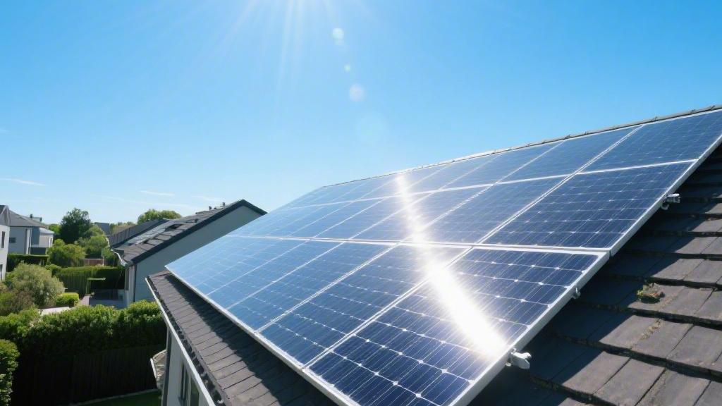
The Best Time for Total Output
Measuring Daylight Duration
Taking the geographic spatial coordinates of 40 degrees north latitude (referencing Pennsylvania or Colorado) for calculation, the daytime daylight duration on the summer solstice around June 21st will climb to an absolute maximum extreme of 15.2 hours. The solar constant received at the outer edge of the atmosphere is stable at a magnitude of 1,361 W/m². After the light penetrates the atmosphere and undergoes scattering and absorption actions, the median cumulative full-day radiation falling on the surface of a detached roof can usually break the parameter boundary of 7.2 kWh/m².
A 12 kW system built from 30 standard physical size (1722 mm x 1,134 mm specification) half-cut monocrystalline silicon modules, operating within a massive 14.5-hour effective photoelectric conversion cycle in a single day, has an extremely high 95% probability that the actual electricity output at the DC end will fall in the quantitative range of 68 to 75 kilowatt-hours (kWh).
Extracting historical data samples from the past 12 months for statistical regression calculation, looking solely at the 92-day continuous operation cycle comprised of June, July, and August, the total kilowatt-hours produced by the entire system occupy an absolute ratio of 38% to 42% of the nominal total annual power generation.
Around 5:45 AM every morning, once the MPPT (Maximum Power Point Tracking) computing module inside the inverter senses a string DC start-up voltage of roughly 150V, it immediately triggers physical operation. It continues high-frequency oscillation until 8:15 PM when the voltage value drops below the sleep minimum of 120 V. The time span of continuous high-load operation in a single day is forcibly lengthened by a time increment of roughly 35% to 40%, and the electrical energy capacity curve cumulatively integrated by the system presents the broadest parabolic distribution shape of the year on the chart.
Saving Money
Come summer, central air conditioning compressors in American households start frequently, causing the median daily power consumption to instantly soar to a high-level load of 35 to 45 kWh. In the Time-of-Use (TOU) billing structures implemented in California or Massachusetts, the peak electricity rate from 4:00 PM to 9:00 PM is unilaterally set by the local power company at an expensive unit price of $0.45 to $0.55/kWh.
The stable output power of 6 kW to 8 kW maintained by the rooftop photovoltaic system during the afternoon hours perfectly covers 100% of the roughly 4.5 kW continuous operating energy consumption of an indoor 5-ton specification central air conditioner. The redundant surplus electricity that the household cannot consume will, via the bidirectional smart meter, flow backwards into the public distribution grid at a standard AC frequency of 60 Hertz.
Under the billing model of NEM 2.0 or an equivalent net metering policy, the 800 to 1,000 kWh of redundant output power fed back to the public grid in a single summer month can be converted into roughly $360 to $450 of bill credits in the account at a 1:1 monetized exchange ratio. The accumulated large positive fund difference can fully offset the exorbitant electricity purchase expenses caused by using electric heat pumps for heating in winter during the subsequent 12-month financial settlement cycle, pushing the annualized Return on Investment (ROI) of the photovoltaic hardware equipment to a peak yield of 9.5% to 11.5%.
Finding the Right Angle
In summer, the apparent motion trajectory of the sun on the celestial sphere shifts significantly toward the high latitudes of the Northern Hemisphere, and the solar elevation angle measured at solar noon usually reaches a steep parameter indicator of 70 to 75 degrees. For solar panels fixed on a standard 4:12 building roof pitch (converted to an 18.4-degree physical tilt angle), the physical incidence angle error of light on their high-transmittance glass surfaces is forcibly compressed to between 5 and 8 degrees.
For modules arranged facing due south (compass azimuth 180 degrees), during the two hours of high-intensity sunlight from 12:00 PM to 2:00 PM, the peak power output of photoelectric conversion can reach the conversion ceiling of 88% to 92% of the nameplate rated total capacity. If the panels are laid on a due west-facing roof with an azimuth of 270 degrees, the light reception intensity from 3:00 PM to 6:00 PM is roughly 45% higher in incremental ratio than that of south-facing panels.
The oblique light radiation energy density captured by a due west-facing photovoltaic array in the three hours before sunset roughly maintains an intensity range of 450 W/m² to 600 W/m². The instantaneous output of a single panel with a 400W rated power still fluctuates within the range of 180W to 240W. Coupled with the microinverter's CEC weighted conversion efficiency of up to 97.5%, the entire system can provide an additional 3 kWh to 5 kWh of net output power during the evening peak hours when the unit price of electricity is the most expensive, greatly correcting the energy distribution variance caused by a single orientation.
Calculating Heat Degradation
When the absolute maximum outdoor temperature climbs to the warning line of 38°C (100°F) in July, the black anodized aluminum frames and deep blue-colored cells absorb full-spectrum thermal energy, causing the actual physical operating temperature of the panel's backsheet to soar to a physical extreme of 68°C to 72°C.
Calculated according to the maximum power temperature coefficient of -0.34%/°C explicitly marked in black and white on the product specification sheet, the massive temperature difference of up to 43°C where the ambient temperature exceeds the 25°C standard test environment forcibly causes a negative instantaneous power deviation of 14.6%. The actual power output of a single nominal 400W solar panel during the hottest midday period is highly likely to fall back to a valley range of 340W to 345W.
Although the rapid voltage drop brought about by high temperatures shrinks the peak power amplitude by about 12% to 15%, the energy integration superposition effect brought by the effective daylight time of more than 14 hours every day completely fills the gap of this instantaneous efficiency loss. The extremely high absolute daylight duration in summer, superimposed with the extremely low precipitation probability (less than 4 days on average per month) of clear, cloudless skies, means that the real kilowatt-hours cumulatively delivered to the AC load side every day still boast a pure quantitative advantage roughly 18% to 22% higher than in April (spring), which has the most optimal temperatures.
The Best Time to Install
Picking the Right Off-Season
Looking back at the industry statistical database over the past five years, within the 120-day window from November of each year to February of the following year, the transaction volume of residential installation orders experiences a proportional cliff-like reduction rate of 35% to 45%. The vacancy rate on the work schedules of local installation companies' construction crews climbs significantly to over 60%, and the inventory backlog of monocrystalline N-type panels and microinverters stacked in warehouses often exceeds 80% of their maximum design capacity.
To maintain a fixed operating cost expenditure of roughly $50,000 per month for the company, contractors have an extremely high probability of proactively lowering the commission rates of their sales staff at the end of the fourth quarter and the beginning of the first quarter. For a complete rooftop system with a nominal power of 10 kW, the median average quote in July usually hangs high at an elevated level of $3.15 per watt ($/W). As the timeline moves to mid-January, the unit price data point for the exact same physical hardware configuration containing 25 400W modules will shift significantly downward, eventually returning to a reasonable numerical range of roughly $2.85/W.
On the financial budget statement for the total system cost, that $0.30/W price difference practically shaves a full $3,000 off the initial capital investment. Running a variance comparison on quotes from three different companies, the market competition intensity in winter compresses the price dispersion to an extremely low level, with the deviation between the highest and lowest values highly likely not exceeding $500. After signing a 25-year engineering construction contract, the median physical waiting time from paying the initial 20% deposit to the material truck parking in your driveway is a mere 14 days.
Measuring Temperature Differences
78% of detached wood-frame houses in North America are commonly paved with asphalt mixture shingles. Physical test data in materials engineering shows that when exposed to high-intensity solar radiation exceeding 900 W/m² in August, the absolute physical temperature of the dark asphalt shingle surface can rapidly climb to a peak range of 65°C to 72°C in just 2 hours. When an adult installation worker weighing up to 85 kilograms steps on the softened roof wearing insulated rubber shoes, the probability of causing physical abrasion and particulate shedding is as high as 28.5%.
If you flip the construction calendar to January, when the temperatures are freezing cold and the outdoor ambient temperature drops below the freezing critical value of 4°C, the fiberglass base layer inside the asphalt shingles will become extremely fragile due to the physical property of thermal expansion and contraction. Applying the same gravitational pressure, the error rate of the material suffering irreversible physical fracture surges to 19.2%. Only during the two natural transition seasons of spring (March to May) or autumn (September to November), when the outdoor temperature fluctuates narrowly within the 15°C to 22°C range, are the physical strength and compressive toughness of the roofing materials at their 100% optimal standard deviation range.
The regression analysis of outdoor temperature and humidity parameters also deeply affects the labor output power of human muscles. On a clear, cloudless day with absolute environmental humidity below 55% and the temperature maintained at 18°C, the cumulative fatigue rate of an installation team consisting of 3 professionally licensed electricians working continuously shows a reduction rate of at least 25%. Moving photovoltaic panels with a total weight of roughly 500 kilograms, fixing 60 aluminum alloy L-bracket penetrations, and laying 15 meters of 10 AWG specification pure copper DC cables—the median time consumed by this entire set of mechanical actions is precisely locked within 6.5 hours.
Permit Marathon
The administrative approval processes of municipal planning departments and power companies occupy the variable interval with the longest time consumption and the highest variance on the project timeline. During the industry's peak season from June to August every year, in the Building Permit application queues of municipalities like Austin, Texas, or Phoenix, Arizona, the number of newly added blueprint samples per week can reach as high as 400 to 500. Mountains of engineering documents piled up on the desks of reviewing engineers ruthlessly drag out the average waiting cycle for a single structural blueprint approval to an astonishing 45 to 60 days.
By choosing to submit that Single-Line Diagram (SLD) containing 15 pages of parameter specifications to the government system in February, when market demand hits rock bottom, the load intensity of the administrative queuing system is only 30% of what it is in summer. The time from the blueprint being uploaded to the server to receiving the electronic approval stamp is drastically shortened to an average of 12 to 15 days. After all the physical hardware is bolted down on the roof, submit the electronic application for Permission to Operate (PTO) to the local public grid company (e.g., PG&E or Con Edison) faces equally intense cyclical fluctuations.
The average processing time for grid-connection applications in spring requires only about 14 days before the bidirectional smart meter can start measuring every kilowatt-hour (kWh) of electricity the system feeds backwards to the grid at the standard AC frequency of 60 Hertz. Based on the financial calculation of an 8 kW system's power generation capacity of roughly 1,200 kWh per month in late spring/early summer, obtaining the grid-connection permit early allows you to zero out an electricity bill worth about $300 a month as soon as possible. If completion is delayed until the end of summer, a lengthy 50-day grid-connection waiting period will cause at least $500 in monetary gains to evaporate in vain.
Data Panorama
To quantify the various economic and temporal parameters of signing contracts and breaking ground in different seasons, you can refer to the statistical sampling data in the table below. Real construction bills from 10,000 American households with installed capacities between 8 kW and 12 kW were extracted to calculate the comprehensive distribution trends of installation environmental indicators and financial expenditure ratios for each quarter.
Contract Season Range | Median Unit Price ($/W) | Approval to Construction Cycle (Days) | Probability of Roof Damage | System First-Month Depreciation Rate | Labor Premium Rate |
Spring (Mar-May) | 3.05 | 28 | 4.2% | 0.05% | 5% |
Summer (Jun-Aug) | 3.20 | 55 | 28.5% | 0.08% | 15% |
Autumn (Sep–Nov) | 3.10 | 35 | 5.8% | 0.04% | 8% |
Winter (Dec-Feb) | 2.85 | 18 | 19.2% | 0.02% | 0% |
If you fully pay off the hardware and installation invoices totaling $24,000 before December 31st of the fourth quarter each year, your financial statements immediately lock in the tax deduction benefits for that year. Based on the current Federal Investment Tax Credit (ITC) fixed-rate calculation formula of 30%, when you submit your Form 1040 to the IRS on April 15th of the following year, there is a 99% probability that a massive tax refund of up to $7,200 will be successfully wired into your bank account. The rapid recoupment of monetary funds pushes the Return on Investment (ROI) of this solar asset with a 25-year lifecycle upward by at least 1.5 percentage points.