Two rear sensors can read 186 W/m² and 189 W/m²—a difference of only 1.6%—while two separately tested modules show Isc values of 13.8 A and 13.2 A, a difference of about 4.3%. If that happens, the rear irradiance reading is only part of the answer. The practical checks are the current metric, front irradiance, Isc bifaciality, rear-light distribution across the module, shading, temperature, timestamps, and measurement uncertainty.
There is one case that should be considered separately from the start. If both modules are operating in the same conventional series string, they carry the same string current. A weaker module will usually show up as lower voltage, lower power, a different I-V curve, bypass activity, or a different result when the module is tested on its own.
Confirm the Current Metric
A bifacial module has one electrical output. There is no separate cable for front-side current and rear-side current.
In real projects, the term “rear-side current” is used in several ways:
- rear-side Isc measured under controlled rear illumination;
- the increase in Isc after rear illumination is added;
- a calculated rear-current contribution;
- or, less precisely, total module current while both sides are illuminated.
Once front and rear light are present at the same time, the value measured at the terminals is total module current.
IEC TS 60904-1-2:2024+AMD1:2026 covers the additional I-V measurement requirements for bifacial PV devices, including rear illumination, irradiance non-uniformity, bifaciality, and equivalent irradiance.[1]
| Isc | Irradiance and photocurrent comparison |
| Imp | Maximum-power operating current |
| Pmax | Actual module power comparison |
| String current | Current through a complete series string |
Compare Isc Bifaciality
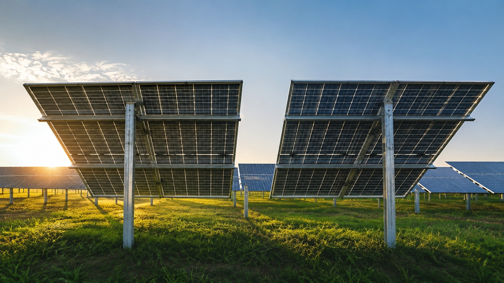
If two modules see the same rear irradiance but have different Isc bifaciality, their rear-side photocurrent response will not be the same.
For short-circuit current:
\[ \phi_{Isc}=\frac{I_{sc,rear}}{I_{sc,front}} \]
Take a module with:
- Front Isc = 14.0 A
- Rear Isc = 11.2 A
\[ 11.2/14.0=0.80 \]
Its Isc bifaciality is 80%.
Now put two simplified modules under the same 200 W/m² rear irradiance:
| Parameter | Module A | Module B |
|---|---|---|
| Front Isc at 1,000 W/m² | 14.0 A | 14.0 A |
| Isc bifaciality | 70% | 90% |
| Rear-equivalent Isc at 1,000 W/m² | 9.8 A | 12.6 A |
| Estimated contribution at 200 W/m² | 1.96 A | 2.52 A |
The estimated difference is:
\[ 2.52-1.96=0.56A \]
The 70% and 90% values above are illustrative values used to show the effect clearly. The exact bifaciality must come from the product's test data.
This is also a first-order estimate. It assumes similar temperature, spectrum, light angle, and rear-light distribution.
The Tongwei TNC-G12R bifacial cell data, for example, shows normalized Isc values of 1.000, 0.903, 0.803, 0.602, and 0.403 at 1,000, 900, 800, 600, and 400 W/m². Under controlled conditions, Isc follows irradiance closely.
When the comparison is about short-circuit current, use the Isc bifaciality value rather than substituting Pmax bifaciality. The current IEC method specifies Isc bifaciality for equivalent-irradiance calculation.[2]
Measure the Rear-Irradiance Spread
The average can look perfectly normal even when part of the module is much brighter or darker than the rest.
| Rear Measurement Point | Module A | Module B |
|---|---|---|
| 1 | 176 W/m² | 260 W/m² |
| 2 | 181 W/m² | 220 W/m² |
| 3 | 180 W/m² | 180 W/m² |
| 4 | 183 W/m² | 140 W/m² |
| 5 | 180 W/m² | 100 W/m² |
| Average | 180 W/m² | 180 W/m² |
Module A range:
\[ 183-176=7W/m^2 \]
Module B range:
\[ 260-100=160W/m^2 \]
Both modules average 180 W/m². Electrically, though, the second module is working under a much more uneven light pattern.
NREL research found that non-uniform rear irradiance creates additional electrical mismatch in bifacial PV. In the systems studied, very low-clearance rooftop configurations showed annual mismatch losses as high as about 2%, while higher-clearance systems were below 0.5%. The same work linked mismatch strongly to the spatial variation of cell-level irradiance.[3]
The max-to-min range is useful for a quick site check, but it does not describe the whole pattern. A full engineering review may use standard deviation, mean absolute difference, or another measure that includes all measurement points.
Use More Than One Rear Measurement Point
A center-mounted sensor can read 205 W/m² while the module actually looks like this:
- upper cell area: 255 W/m²;
- center cell area: 205 W/m²;
- lower cell area: 125 W/m².
The sensor value itself looks reasonable, but the rear-light spread is:
\[ 255-125=130W/m^2 \]
That difference would be invisible if the diagnosis relied only on the center sensor.
For module-level troubleshooting, useful positions include:
- upper area;
- center;
- lower area;
- an area near a torque tube, rail, or other suspected obstruction.
Module height, tracker angle, row spacing, ground shadow, torque-tube position, and nearby structures can all change the rear-light pattern from one part of the module to another.
Check Series-Cell Mismatch
Suppose six cells would produce these currents if each could work independently:
- 6.0 A
- 6.1 A
- 5.9 A
- 6.0 A
- 3.8 A
- 6.0 A
The electrical result is not the simple average:
\[ (6.0+6.1+5.9+6.0+3.8+6.0)/6=5.63A \]
It is also not accurate to treat the group as a fixed 3.8 A source.
Cells in the same series path have to carry a common current. The weakly illuminated cell changes the voltage balance of the group and pulls the other cells away from the operating points they would have under even light.
Sandia PVPMC describes the same effect for series-connected PV devices: differences in irradiance, temperature, or electrical characteristics create mismatch because connected devices cannot all remain at their own maximum-power points.[4]
Depending on how severe the mismatch becomes, the module may show:
- lower voltage;
- lower Pmax;
- a distorted I-V curve;
- reverse bias in strongly affected cells;
- bypass-diode operation.
Match the Shadow to the Cell Layout
A 10% shadow is not a complete description of the electrical problem. Where that 10% falls can change the result.
| Shadow A | Shadow B | |
|---|---|---|
| Approximate shaded area | 10% | 10% |
| Shape | Narrow strip | Concentrated block |
| Likely electrical effect | Touches several strings | May strongly affect one substring or branch |
Modern modules can use half-cut cells, several series substrings, parallel branches, and multiple bypass diodes. A shadow crossing several strings is not the same electrical event as a shadow concentrated on one substring.
NREL's bifacial modeling tools include racking geometry, partial shading, cell-level mismatch, and half-cell module behavior because these details change the electrical result.[5]
For a real project, the module drawing and electrical layout are worth checking. Tongwei's module technical data, for example, lists cell arrays, Isc, Imp, Vmp, and junction-box diode counts for different module configurations.
Look for Bypass-Diode Signatures
Small rear-light differences usually create mismatch before they create bypass-diode conduction.
Suppose a module normally operates around:
\[ V_{mp}=42V \]
If one protected substring becomes bypassed, Vmp can fall by many volts. The exact drop depends on the module circuit and should not be assumed to equal exactly one-third of the module voltage.
NREL tests on partially shaded crystalline-silicon systems showed that a relatively small physical shadow can create a power loss much larger than the shadow area itself because series connection and bypass behavior magnify the electrical effect.[6]
Bypass behavior deserves attention when the field data show:
- a clear step in the I-V curve;
- a large Vmp drop;
- power loss much larger than expected from the shaded area;
- a problem that appears only at specific tracker angles.
Separate Isc, Imp, Vmp, and Pmax
Current by itself does not tell you how much power the module is producing.
\[ P=V\times I \]
| Current | Voltage | Power | |
|---|---|---|---|
| Module A | 10.0 A | 40.0 V | 400 W |
| Module B | 9.7 A | 41.3 V | 400.61 W |
Module B has 3% lower current but virtually the same power.
| Metric | Best Use |
|---|---|
| Isc | Compare photocurrent and irradiance response |
| Imp | Compare current near maximum power |
| Vmp | Find voltage loss, mismatch, or bypass effects |
| Pmax | Compare total module power |
Check Front Irradiance
Rear readings can match while the total light on the two modules is still different.
A simple front-equivalent comparison is:
\[ G_{eq}\approx G_f+\phi_{Isc}G_r \]
Assume both modules have 80% Isc bifaciality:
| Module A | Module B | |
|---|---|---|
| Front irradiance | 900 W/m² | 850 W/m² |
| Rear irradiance | 200 W/m² | 200 W/m² |
| Isc bifaciality | 80% | 80% |
Module A:
\[ 900+(200\times0.80)=1060W/m^2 \]
Module B:
\[ 850+(200\times0.80)=1010W/m^2 \]
The rear sensors match, but the simplified front-equivalent irradiance differs by:
\[ 1060-1010=50W/m^2 \]
Relative to Module A:
\[ 50/1060\approx4.7\% \]
With a gap of this size, equal independently measured Isc would not be the expected result.
Treat Spectrum and Light Angle as Secondary Checks
Spectrum and sensor type matter, but they normally come later in the troubleshooting order. First rule out larger causes such as front irradiance, bifaciality, shading, and rear non-uniformity.
A thermopile pyranometer measures broadband solar radiation. A silicon reference device responds more like a silicon PV device.
NREL research on bifacial measurements found that spectral effects can make measured rear irradiance differ from PV-effective irradiance. In the modeled cases reported in the study, the deviation was on the order of 16.5 W/m² for a pyranometer and 3.6 W/m² for a PV reference cell.[7]
Ground material changes the reflected spectrum as well. Snow, grass, soil, concrete, sand, and gravel do not reflect every wavelength in the same way.
PV current depends on the incoming spectrum and the cell response:
\[ I_{sc}\propto\int E(\lambda)SR(\lambda)d\lambda \]
Light angle is another part of the same picture. If a problem becomes stronger only in the morning, afternoon, or at specific tracker positions, check geometry and shading before treating the module itself as faulty.
Sandia's effective-irradiance framework accounts for factors such as angle of incidence, soiling, and spectral mismatch.[8]
Quantify the Temperature Effect
Temperature should be calculated, not guessed.
Assume:
\[ \alpha_{Isc}=+0.05\%/^{\circ}C \]
| Cell-Temperature Difference | Approximate Isc Effect |
|---|---|
| 5°C | 0.25% |
| 10°C | 0.50% |
| 20°C | 1.00% |
If Isc differs by 6%, a 5–10°C temperature gap is not enough to explain the whole difference.
Tongwei's current module technical data lists an Isc temperature coefficient of about +0.046%/°C for several TNC module configurations, which is close to the 0.05%/°C example used above.
Use module or cell temperature for this check. Ambient temperature does not tell you the actual cell temperature.
Separate Soiling From Moving Shade
A quick way to separate these two causes is to watch whether the pattern moves.
| Pattern | More Likely Cause |
|---|---|
| Loss stays in the same place for days | Soiling or fixed obstruction |
| Loss moves during the day | Structural shadow |
| Loss appears at one tracker angle | Torque tube, rail, purlin, or nearby row |
| Sensor looks low but module performs normally | Check sensor cleanliness or calibration |
A clean rear sensor can read 190 W/m² while dirt on the module reduces the light entering the rear surface. A dirty sensor can create the opposite error.
For Tongwei modules, cleaning and inspection should follow the current module installation and maintenance documentation.
Match the Timestamps
A five-minute irradiance average is not the same thing as the irradiance during a one-second I-V measurement.
Example rear irradiance during five minutes:
150 → 230 → 170 W/m²
The simple average is about:
183 W/m²
If the I-V curve was captured at 230 W/m², the instantaneous value was:
\[ 230-183=47W/m^2 \]
above the logged average.
That is approximately:
\[ 47/183\approx25.7\% \]
A gap this large is more than enough to distort a module-to-module comparison.
Use matching timestamps for:
- front irradiance;
- rear irradiance;
- module temperature;
- I-V data.
Compare the Gap With Test Uncertainty
Small differences should be compared with the accuracy of the whole test setup.
Suppose two adjusted Isc measurements are:
- 13.80 A;
- 13.66 A.
The difference is:
\[ \frac{13.80-13.66}{13.80}\times100\%\approx1.0\% \]
If the complete measurement uncertainty is about ±2%, that 1% gap is not strong evidence that one module is electrically worse.
The uncertainty check should include:
- irradiance-sensor calibration;
- sensor position;
- temperature measurement;
- I-V tracer accuracy;
- spectral response;
- timestamp mismatch.
The current IEC specification states that spectral mismatch correction is not mandatory in every bifacial I-V measurement unless required by another standard, but spectral mismatch still has to be included in the measurement uncertainty.[9]
Confirm Whether the Modules Share One Series Current
For two modules in the same conventional series string:
\[ I_A=I_B=I_{string} \]
They cannot simultaneously carry independent string currents of 12 A and 10 A.
When one module is weaker, the difference is more likely to appear as:
- lower module voltage;
- lower string power;
- a stepped I-V curve;
- bypass-diode activity;
- local heating.
If the monitoring system shows different module-level current values inside one string, first check where those numbers come from. They may be produced by optimizers, module-level electronics, individual tests, or software calculations.
Compare Like With Like
Rated wattage alone is not enough to compare two module designs.
For different models, compare:
- front Isc;
- Isc bifaciality;
- Imp;
- Vmp;
- cell arrangement;
- junction-box diode count.
Tongwei's current module data includes bifacial configurations with different cell arrays and electrical values. Its TNC-G12 66 bifacial series, for example, lists Isc values in the roughly 18.35–18.55 A range across the shown power classes, which is why two modules with similar wattage should not be assumed to have the same current.
Model-specific documents can also be checked through Tongwei's technical download library.
Normalize Before Judging the Module
Raw data can make a normal module look worse than it is.
Example raw values:
- Module A Isc = 13.8 A
- Module B Isc = 13.1 A
Raw difference:
\[ \frac{13.8-13.1}{13.8}\times100\%\approx5.1\% \]
After adjusting for irradiance and temperature, suppose the values become:
- Module A adjusted Isc = 13.75 A
- Module B adjusted Isc = 13.68 A
Adjusted difference:
\[ \frac{13.75-13.68}{13.75}\times100\%\approx0.5\% \]
In this example, the original 5.1% gap falls to about 0.5% after the test conditions are corrected.
For warranty, certification, or contractual acceptance testing, use the applicable standard procedure and full uncertainty calculation rather than a simple field adjustment.
Require Repeatable Results
| Module A | Module B | |
|---|---|---|
| Test 1 | 13.8 A | 13.3 A |
| Test 2 | 13.5 A | 13.7 A |
Module B is lower in Test 1, but Module A is lower in Test 2. That pattern does not point to a stable fault in one specific module.
A result becomes more meaningful when:
- the same module is lower in repeated tests;
- front and rear irradiance are comparable;
- temperature has been corrected;
- timestamps match;
- the difference remains larger than expected test uncertainty.
Use the I-V Curve to Separate Causes
Assume a healthy comparison module under one test condition gives:
- Isc = 14.0 A
- Voc = 50.0 V
- Imp = 13.2 A
- Vmp = 45.5 V
- Pmax ≈ 600 W
| Measured Pattern | Illustrative Data | Check First |
|---|---|---|
| Lower Isc, smooth curve | Isc 13.2 A, Pmax ≈565 W | Irradiance, soiling, sensor error |
| Similar Isc, lower Pmax | Isc 13.9 A, Pmax ≈550 W | Mismatch, series resistance, temperature |
| Curve has a clear step | Isc ≈13.8 A, Vmp roughly 31–35 V | Substring shading or bypass operation |
| Voc unusually low | Clearly below the comparison module | Temperature, failed diode, inactive cells, measurement error |
The numbers above are examples, not universal fault limits.
One useful clue is the relationship between current loss and power loss. If Isc changes from 14.0 A to 13.9 A—a reduction of only about 0.7%—while Pmax drops from 600 W to 550 W, or about 8.3%, a small rear-irradiance difference is unlikely to explain the whole result.
Use This Diagnostic Order
- Identify whether the value is Isc, Imp, Pmax, or string current.
- Confirm whether the modules are the same model.
- Compare front irradiance.
- Compare Isc bifaciality.
- Measure rear irradiance at several positions.
- Check the max-to-min spread and the location of low-irradiance cells.
- Inspect torque tubes, rails, piles, and nearby rows.
- Measure module temperature.
- Check the module and sensor for dirt.
- Match irradiance and I-V timestamps.
- Compare the observed gap with test uncertainty.
- Normalize the data and repeat the measurement.
- If the same abnormality remains, inspect the full I-V curve.
Worked Example: Rear Sensors Match, Isc Does Not
The numbers below are a hypothetical diagnostic example.
| Measurement | Module A | Module B |
|---|---|---|
| Front irradiance | 900 W/m² | 902 W/m² |
| Center rear sensor | 185 W/m² | 187 W/m² |
| Module temperature | 43°C | 44°C |
| Isc | 13.9 A | 13.1 A |
Rear-sensor difference:
\[ \frac{187-185}{185}\times100\%\approx1.1\% \]
Isc difference:
\[ \frac{13.9-13.1}{13.9}\times100\%\approx5.8\% \]
The 1.1% center-sensor gap is too small to explain a 5.8% current gap on its own.
Now measure five rear positions:
| Module A | Module B | |
|---|---|---|
| Point 1 | 180 W/m² | 105 W/m² |
| Point 2 | 183 W/m² | 142 W/m² |
| Point 3 | 185 W/m² | 188 W/m² |
| Point 4 | 188 W/m² | 228 W/m² |
| Point 5 | 189 W/m² | 272 W/m² |
| Average | 185 W/m² | 187 W/m² |
| Range | 9 W/m² | 167 W/m² |
Module B does not have meaningfully lower average rear irradiance. The real difference is that its rear light is far less uniform.
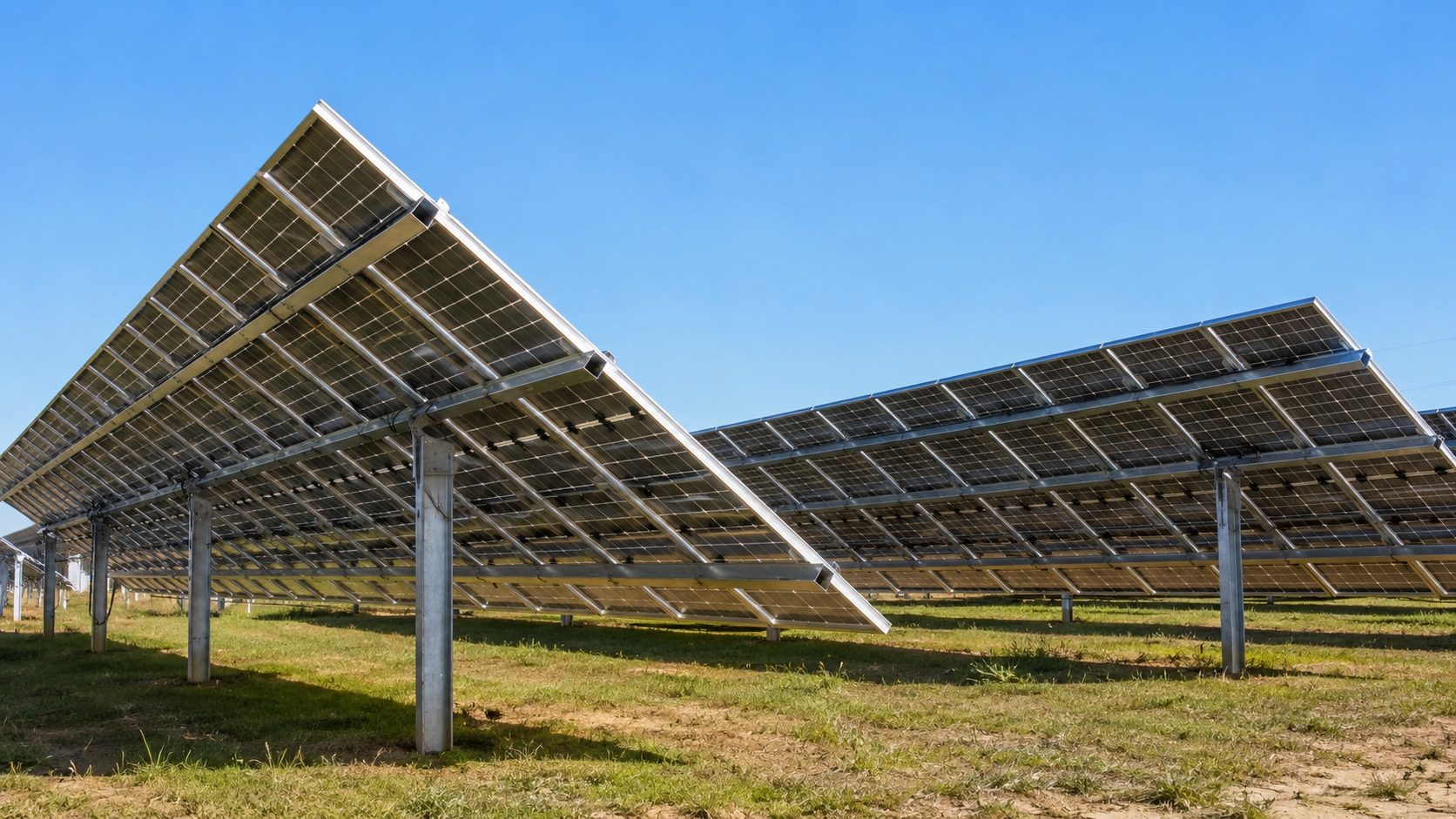
If the 105–142 W/m² area lines up with a torque tube, rail, or other structure, rear-side mismatch becomes a much stronger explanation than a defective module. The sensible next step is to repeat the test and compare the I-V curves before making a module-fault decision.
Escalate to Module-Fault Checks Only After Normalization
Move to module-fault checks when most of the basic test conditions have already been ruled out:
- the modules are the same model and power class;
- front irradiance is comparable;
- rear-light distribution has been measured;
- temperature has been corrected;
- sensor and timestamp problems have been ruled out;
- the test has been repeated;
- the same module remains abnormal.
| Possible Problem | More Typical Sign |
|---|---|
| High series resistance | Lower fill factor, Vmp, and Pmax; Isc may remain close to normal |
| High-resistance connector | Voltage drop and heat under load |
| Electrically significant cell crack | Inactive cell area or abnormal I-V response |
| Shorted bypass diode | Abnormally low module voltage |
| Partial shading | Mismatch, I-V steps, possible bypass operation |
Before a warranty or laboratory investigation, collect the module model and serial number, front and rear irradiance, module temperature, I-V curves, timestamps, photos, tracker position, and cleaning history.
Finally
If two rear sensors both read about 180–200 W/m² but separately measured Isc differs by 4–6%, do not judge the modules from the rear-sensor value alone. Compare front irradiance and Isc bifaciality, then check rear irradiance at several cell positions. A module averaging 180 W/m² with a 7 W/m² spread is not in the same electrical condition as one averaging 180 W/m² with a 160 W/m² spread. Correct temperature and timing differences, compare the gap with test uncertainty, and repeat the test. A module-level fault becomes credible only when the same abnormal I-V result remains after those checks.
Safety note: Do not disconnect live PV connectors, intentionally short-circuit operating modules to measure Isc, or open energized junction boxes unless you are qualified to work on PV DC systems. For Tongwei modules, follow the current installation and maintenance instructions.