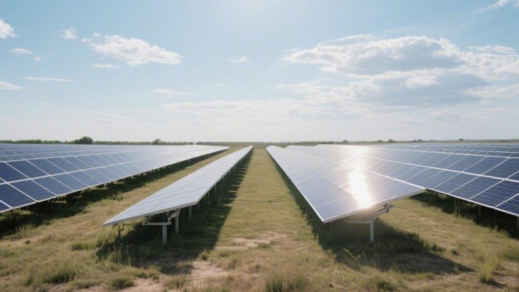
What is the minimum distance between rows of solar panels

The minimum row spacing should be 2.5 times the height of the array to ensure no shading between 10:00 AM and 2:00 PM on the Winter Solstice.

During operation, field measurements of shadow length are required, and an O&M corridor of approximately 4-6 meters should be reserved between arrays.

Using the formula D = H x 2.5 balances land utilization with generation efficiency, ensuring the stable operation of the power plant for 25 years.

Performance & Shading

A Bit of Shade, A Year's Loss

In a series circuit, if 10% of the bottom area of a single 550W module is shaded by the front row, the current output of the entire string of 26 modules will be forced down to the level of that shaded panel. This results in an instantaneous power drop of over 85% for the entire string. This "bucket effect" is most lethal between 8:00 AM and 10:00 AM. If the row spacing is reduced by 0.5 meters to save 15% of land area, the cumulative annual energy loss will reach 4.2% to 6.8%. For a 1MW distributed project, this 0.5-meter spacing deviation will lead to a loss of 2.1 million kWh over a 25-year cycle, equivalent to a financial loss of approximately $1.2 million to $1.8 million in electricity revenue.

We must also pay attention to the frequency of bypass diode activation. When shading covers a cell, the diode bypasses that section to protect the circuit; while this prevents hot-spot burnout, it causes an immediate jump in output voltage. Typically, a three-stage diode design results in a one-third loss of voltage if one-third of the cells are shaded. In high-latitude regions, if the effective sunshine window on the winter solstice is compressed from 6 hours to 4.5 hours due to shading, the system efficiency (PR value) will drop from a standard 80% to below 72%, and the Internal Rate of Return (IRR) will decrease by 1.5 to 2 percentage points.

Accurate Shadow Coefficient

In practical engineering at 37 degrees north latitude, we utilize the "shadow coefficient" as a quantitative indicator. Simply put, if the highest point of your rack is 1.5 meters above the ground, its shadow length at 9:00 AM on the winter solstice is approximately 3.45 meters. The coefficient here is 2.3x. If the coefficient is forced down to 1.8x to pursue higher installation density, your rear modules will enter full shading after 2:30 PM throughout December and January. During this time, the inverter will frequently perform MPPT optimization due to voltage fluctuations, resulting in an additional 0.5% to 1.2% loss in standby power consumption.

Specific physical spacing calculations cannot rely solely on ground distance; one must look at the horizontal projection from the front edge to the rear edge of the array. For a 2.28-meter-long module installed at a 30-degree tilt, its horizontal projection width is 1.97 meters and its vertical height is 1.14 meters. To ensure 6 hours of shade-free operation on the winter solstice, the total row spacing (including the projection width) usually needs to reach 4.8 to 5.2 meters. Under this configuration, the installed capacity per hectare is approximately 0.6 MW to 0.8 MW. Only when land lease costs exceed 15 RMB per square meter per year do we consider reducing the installation angle by 5 degrees to shrink the spacing by 10%, thereby balancing per-watt cost with total yield.

Efficiency and Heat

Shading affects more than just current; it induces the hot-spot effect. When part of a solar cell becomes a load due to shading, its local temperature can soar from 45°C to over 85°C within 3 minutes. This 40-degree temperature difference leads to accelerated aging of the encapsulation material (EVA), with the yellowing rate increasing threefold, and the annual degradation rate of the module increasing from the nominal 0.45% to 0.8% or higher. Long-term exposure to such localized overheating can shorten the power warranty from 25 years to around 18 years, effectively causing 28% of the asset value to evaporate.

To optimize performance, we compare ventilation efficiency under different spacing. When the row spacing is increased from 2 meters to 4 meters, the wind speed between arrays increases by 25%, which can carry away 3 to 5 degrees of heat from the module backsheet. According to the physical characteristics of silicon-based cells, for every 1-degree drop in operating temperature, the output power increases by approximately 0.35%. During high-temperature periods in summer, the ventilation benefits of wide spacing can increase daily system generation by 1.5% to 2.2%. When evaluating spacing, this "temperature rise benefit" must be factored into the 25-year total ledger.

Avoiding Inefficient Zones

During early morning and late evening, when the solar elevation angle is low, the proportion of diffuse light increases from 15% to over 40%. If the spacing is too narrow, not only is direct light blocked, but the module's ability to capture reflected and diffuse light from the surrounding environment also drops by 5% to 10%. For bifacial modules, the rear-side gain is highly dependent on ground reflection. If narrow spacing causes the ground to remain in shadow for long periods, the albedo (reflectivity) will drop from 20% for dry soil to below 8%, causing the bifacial gain to shrink from an expected 10% to less than 3%.

In actual O&M, spacing also affects cleaning frequency. Narrow spacing prevents O&M vehicles from passing, forcing reliance on manual labor to drag water hoses, which increases cleaning costs from 0.02 RMB to 0.05 RMB per watt. Shading caused by dust accumulation due to inconvenient cleaning results in a 2% to 3% monthly power loss. In high-dust areas, if a 3.5-meter automated cleaning corridor is sacrificed to install 10% more panels, the composite power loss from dust and mutual shading often exceeds the gains from the extra panels, extending the overall investment payback period by 14 to 18 months.

Land ROI

Trading Space for Gold

Typically, the Ground Coverage Ratio (GCR) of a standard power plant is set between 30% and 50%. If we compress the row spacing from 6 meters to 4.5 meters, the installed capacity for the same piece of land can increase by 25% to 33%. In terms of initial investment, while land lease costs remain constant, the land cost amortization per watt decreases by about 20%. For a project with a lease cost of $2,000 per hectare per year, a high-density layout can dilute the land cost per kWh from 3% to approximately 2.2%. However, this increase in capacity is not without cost.

Due to mutual shading caused by reduced spacing, the average annual utilization hours per module will decrease by 40 to 70 hours. Over a 25-year lifecycle, this small annual loss produces a compounding effect. If the feed-in tariff is $0.05/kWh, a 10MW project that loses 5% of total generation due to excessive density will see $75,000 of cash flow evaporate annually. According to IRR modeling, when the power loss from shading exceeds 6.2%, the marginal revenue from increased capacity is completely offset by maintenance costs and generation reduction, extending the overall payback period from 7.2 years to over 8.5 years.

Saving Money with Proper Roads

In large-scale power plants, if the row spacing is below 3 meters, large automated cleaning vehicles and mowers will be unable to enter. The cost of manual cleaning is usually 0.04 to 0.06 RMB per watt, whereas using vehicle-mounted mechanical cleaning can drive this cost down to 0.012 to 0.02 RMB. For a 50 MW project cleaned four times a year, the O&M cost savings from proper spacing can reach 600,000 to 800,000 RMB.

Core Data Quote: On flat terrain, increasing the corridor width from 2.5 meters to 3.5 meters may lose about 8% of theoretical installed capacity, but it improves O&M efficiency by 40%. In arid regions with heavy dust accumulation, the 3.5% to 5% generation gain from timely cleaning compensates for the reduced capacity and lowers the LCOE by approximately 0.005 RMB.

Furthermore, considering long-term land leveling and vegetation management, wide spacing allows for the operation of small agricultural machinery. If insufficient spacing is left and the frequency of manual mowing cannot keep up with plant growth, the hot-spot effect caused by weeds shading the bottom cells will result in an additional 0.2% annual degradation. This hidden cost is often ignored in financial reports, but it can slash the residual value of the asset by over 15% by year 20.

Getting More from the Rear Side

The rear side of bifacial modules absorbs reflected light from the ground, which typically accounts for 5% to 15% of total power. Experimental data shows that when row spacing is stretched from 4 meters to 8 meters, the total amount of diffuse and reflected light received by the rear side increases by 30% to 45%. In environments with light-colored soil or gravel (Albedo approx. 25% to 30%), the rear-side gain from such spacing can increase total plant generation by about 3.2%.

Spacing Width	Density (MW/Hectare)	Bifacial Gain Ratio	25-Year Total Revenue Change
4.0 m	0.85	4.5%	Baseline
5.5 m	0.68	8.2%	Increased by 1.2%
7.0 m	0.55	11.5%	Decreased by 4.8% (Capacity loss too high)

As seen from the table, the optimal ROI solution typically appears in the 5 to 6-meter range. Within this range, the non-linear growth of bifacial gain effectively compensates for the loss in capacity. If single-axis tracking racks are used, spacing requirements become even stricter, usually requiring a center-to-center distance of over 6.5 meters to avoid severe mutual shading when the racks rotate to large angles (e.g., 45 to 60 degrees). The PR value of systems in this configuration can usually be maintained at a high level of over 82%.

Rent Determines Width

If an agreement is charged based on installed capacity (per kW), the design tends toward wider spacing to pursue the highest yield per watt; if the agreement is based on land area (per acre or hectare), the design tends toward tighter spacing. In areas where land rent exceeds $1,500 per acre, developers often choose a 35-degree or even higher tilt combined with a more compact layout, sacrificing 2% in shading loss to gain 10% in installation capacity, thereby reducing the per-watt land cost burden.

We also need to quantify land leveling costs (CAPEX). On complex terrain with slopes exceeding 5 degrees, increasing row spacing requires more earthwork to ensure the elevation of each rack row remains consistent. The cost of excavation and backfilling is approximately 15 to 30 RMB per cubic meter. If spacing is widened to pursue absolute zero-shading, resulting in a 15% increase in DC cable usage, it not only increases copper procurement costs but also raises DC-side line losses from a standard 1% to 1.4%. The cumulative power loss from this 0.4% line loss over 20 years is enough to offset the light gain from an extra 0.5 meters of spacing.

Maintainability

When designing large-scale PV plants over 10 MW, setting row spacing between 3.5 and 4.0 meters allows for automated cleaning vehicles (2.8 m wide) to travel at a constant speed of 5 km/h. Under this mechanized mode, a single piece of equipment can clean 1.5 MW of modules per day, a 400% efficiency increase compared to manual labor at 0.8-meter spacing.

If the spacing is compressed to below 2.5 meters, large vehicles cannot enter, and one must rely on small 1.2-meter robots or manual hose dragging, causing the cleaning price per watt to rise from 0.015 RMB to 0.045 RMB. In a 10MW project with 18,182 modules (550W), cleaning 4 times a year with improper spacing leads to an extra 120,000 to 180,000 RMB in annual O&M expenses.

A properly reserved 3.8-meter corridor also ensures that 5-ton maintenance vehicles can reach deep into the arrays, shortening material transport time from 2 hours to 15 minutes during inverter or transformer failures, thereby increasing the system's annual effective utilization hours by 0.5%.

A single 550W module typically measures 2.28m x 1.13m and weighs approximately 32.3 kg, requiring two workers for replacement. If a net space of over 1.2 meters is left in the row spacing, workers have a 360-degree rotation radius while carrying the 2-meter-long panel, keeping replacement time per panel under 20 minutes.

When spacing is below 0.6 meters, workers must carry the 32 kg load sideways. This extends the replacement time to 45 minutes and increases the probability of micro-cracks in adjacent modules by about 12% due to restricted space. Over a 25-year period, the annual failure rate of modules is typically 0.1% to 0.3%; for a 100 MW project, 180 to 540 panels need replacement annually.

If narrow spacing leads to a 50% increase in labor costs plus a 5% secondary damage rate, the present value loss of long-term O&M costs will reach 800,000 to 1.1 million RMB. Additionally, a 1.5-meter maintenance path allows for the use of hydraulic lift platforms, reducing the risk of falls by over 75% when personnel check wiring at the top of 1.8-meter racks.

Vegetation management under PV arrays is critical for fire prevention and shading protection; row spacing directly determines the selection and frequency of mowing equipment. Spacing above 3.0 meters allows for 1.5-meter-wide ride-on mowers, which work at 6 acres per hour at a cost of about 45 RMB per acre.

If the spacing is only 1.5 meters, only handheld mowers can be used, with efficiency dropping to 0.8 acres per hour and costs soaring to over 180 RMB per acre. In areas with high precipitation requiring 3 to 5 weedings a year, a 1.5-meter difference in spacing can lead to a 25% to 40% deviation in cumulative 20-year O&M costs.

If vegetation height exceeds 0.5 meters and shades the bottom cells, it triggers bypass diodes, reducing string voltage by 33.3%. Long-term shading creates local hot spots exceeding 85°C, raising the annual degradation rate from a normal 0.45% to over 0.95%, causing power revenue to shrink by about 15% after the 10th year.

To quantify the impact of different spacing on maintenance costs, refer to the following 25-year cycle data model. This model assumes a 10 MW plant capacity using 550 W monocrystalline modules.

Physical Spacing (m)	O&M Tool Type	Annual O&M Cost (RMB/W)	25-Year Cumulative OPEX (10k RMB)	Fault Response Time (Hours)
1.5 m	Manual + Small tools	0.08	2000	48
2.5 m	Small robots + Narrow vehicle	0.05	1250	24
4.0 m	Large automated vehicles	0.02	500	4

As shown in the table, increasing spacing from 1.5 meters to 4.0 meters reduces cumulative 20-year O&M costs by 75%, even if land rent increases by 15% to 20%. Considering that DC-side cable losses are typically controlled within 1.5% and AC-side losses are 0.5%, wide spacing significantly aids in improving the system PR value (Performance Ratio).

Adding 2 meters to row spacing also helps keep rack structures stable under Level 12 wind gusts by reducing the turbulence effect between arrays by over 15%. This 0.15x reduction in wind load lowers the wear rate of steel racks by 5% over 20 years, extending the lifespan of foundation piles.